机器学习-07-分类回归和聚类算法评估函数及案例
机器学习-07-分类回归和聚类算法评估函数及案例

总结
本系列是机器学习课程的系列课程,主要介绍机器学习中分类回归和聚类算法中的评价函数。
参考
Python sklearn机器学习各种评价指标——Sklearn.metrics简介及应用示例
https://scikit-learn.org/stable/modules/model_evaluation.html
For the most common use cases, you can designate a scorer object with the scoring parameter; the table below shows all possible values. All scorer objects follow the convention that higher return values are better than lower return values. Thus metrics which measure the distance between the model and the data, like metrics.mean_squared_error, are available as neg_mean_squared_error which return the negated value of the metric. 对于最常见的用例,你可以使用scoring参数指定一个分数衡量指标。 下表显示了所有可能的值。 所有分数衡量指标均遵循以下约定:较高的返回值比较低的返回值更好。 因此,用于度量模型预测值与真实数据值之间误差的度量(如metrics.mean_squared_error)使用neg_mean_squared_error,该度量返回度量的取相反数(去相反数就是为了遵守上述约定)。
Scoring | Function | Comment |
|---|---|---|
Classification | ||
‘accuracy’ | metrics.accuracy_score | |
‘balanced_accuracy’ | metrics.balanced_accuracy_score | |
‘top_k_accuracy’ | metrics.top_k_accuracy_score | |
‘average_precision’ | metrics.average_precision_score | |
‘neg_brier_score’ | metrics.brier_score_loss | |
‘f1’ | metrics.f1_score | for binary targets |
‘f1_micro’ | metrics.f1_score | micro-averaged |
‘f1_macro’ | metrics.f1_score | macro-averaged |
‘f1_weighted’ | metrics.f1_score | weighted average |
‘f1_samples’ | metrics.f1_score | by multilabel sample |
‘neg_log_loss’ | metrics.log_loss | requires predict_proba support |
‘precision’ etc. | metrics.precision_score | suffixes apply as with ‘f1’ |
‘recall’ etc. | metrics.recall_score | suffixes apply as with ‘f1’ |
‘jaccard’ etc. | metrics.jaccard_score | suffixes apply as with ‘f1’ |
‘roc_auc’ | metrics.roc_auc_score | |
‘roc_auc_ovr’ | metrics.roc_auc_score | |
‘roc_auc_ovo’ | metrics.roc_auc_score | |
‘roc_auc_ovr_weighted’ | metrics.roc_auc_score | |
‘roc_auc_ovo_weighted’ | metrics.roc_auc_score | |
Clustering | ||
‘adjusted_mutual_info_score’ | metrics.adjusted_mutual_info_score | |
‘adjusted_rand_score’ | metrics.adjusted_rand_score | |
‘completeness_score’ | metrics.completeness_score | |
‘fowlkes_mallows_score’ | metrics.fowlkes_mallows_score | |
‘homogeneity_score’ | metrics.homogeneity_score | |
‘mutual_info_score’ | metrics.mutual_info_score | |
‘normalized_mutual_info_score’ | metrics.normalized_mutual_info_score | |
‘rand_score’ | metrics.rand_score | |
‘v_measure_score’ | metrics.v_measure_score | |
Regression | ||
‘explained_variance’ | metrics.explained_variance_score | |
‘max_error’ | metrics.max_error | |
‘neg_mean_absolute_error’ | metrics.mean_absolute_error | |
‘neg_mean_squared_error’ | metrics.mean_squared_error | |
‘neg_root_mean_squared_error’ | metrics.root_mean_squared_error | |
‘neg_mean_squared_log_error’ | metrics.mean_squared_log_error | |
‘neg_root_mean_squared_log_error’ | metrics.root_mean_squared_log_error | |
‘neg_median_absolute_error’ | metrics.median_absolute_error | |
‘r2’ | metrics.r2_score | |
‘neg_mean_poisson_deviance’ | metrics.mean_poisson_deviance | |
‘neg_mean_gamma_deviance’ | metrics.mean_gamma_deviance | |
‘neg_mean_absolute_percentage_error’ | metrics.mean_absolute_percentage_error | |
‘d2_absolute_error_score’ | metrics.d2_absolute_error_score | |
‘d2_pinball_score’ | metrics.d2_pinball_score | |
‘d2_tweedie_score’ | metrics.d2_tweedie_score |
本门课程的目标
完成一个特定行业的算法应用全过程:
懂业务+会选择合适的算法+数据处理+算法训练+算法调优+算法融合 +算法评估+持续调优+工程化接口实现
机器学习定义
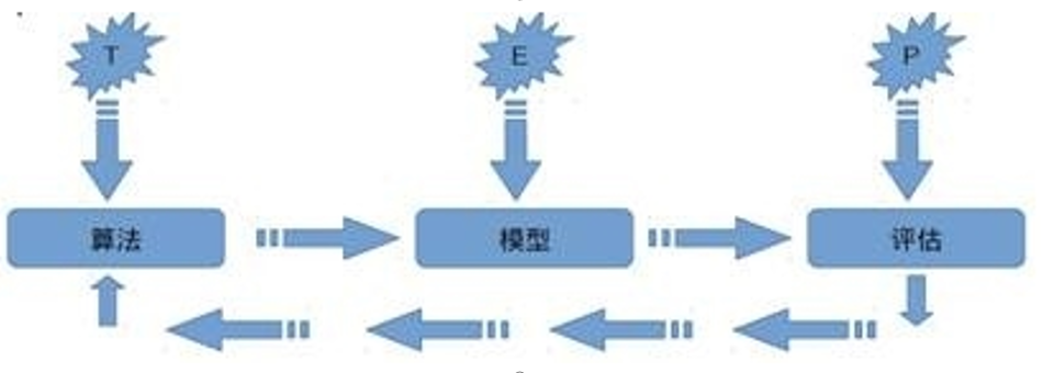
关于机器学习的定义,Tom Michael Mitchell的这段话被广泛引用: 对于某类任务T和性能度量P,如果一个计算机程序在T上其性能P随着经验E而自我完善,那么我们称这个计算机程序从经验E中学习。
机器学习常见评价指标
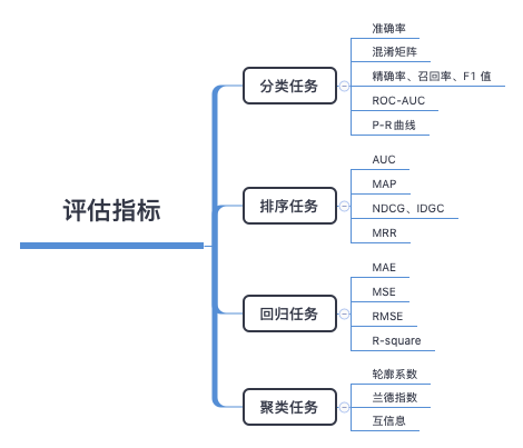
“没有测量,就没有科学。”——门捷列夫 在计算机科学特别是机器学习领域中,对模型的评估同样至关重要。只有选择与问题相匹配的评估方法,才能快速地发现模型选择或训练过程中出现的问题,迭代地对模型进行优化。 本篇文章就给大家分享一下分类和回归模型中常用地评价指标,希望对大家有帮助。
介绍
有三种不同的方法来评估一个模型的预测质量:
estimator的score方法:sklearn中的estimator都具有一个score方法,它提供了一个缺省的评估法则来解决问题。 Scoring参数:使用cross-validation的模型评估工具,依赖于内部的scoring策略。见下。 Metric函数:metrics模块实现了一些函数,用来评估预测误差。见下。
scoring参数
模型选择和评估工具,例如:
from sklearn.model_selection import cross_val_score
 from sklearn.model_selection import GridSearchCV
使用scoring参数来控制你的estimator的好坏。
#导入数据集模块
from sklearn import datasets
#分别加载iris和digits数据集
iris_dataset = datasets.load_iris() #鸢尾花数据集
# print(dir(datasets))
# print(iris_dataset.keys())
# dict_keys(['data', 'target', 'frame', 'target_names', 'DESCR', 'feature_names', 'filename', 'data_module'])
from sklearn.model_selection import train_test_split
X_train,X_test,y_train,y_test=train_test_split(iris.data,iris.target,test_size=0.4,random_state=0)
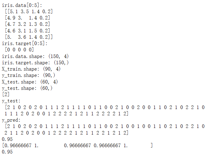
print("iris.data[0:5]:\n",iris.data[0:5])
print("iris.target[0:5]:\n",iris.target[0:5])
print("iris.data.shape:",iris.data.shape)
print("iris.target.shape:",iris.target.shape)
print("X_train.shape:",X_train.shape)
print("y_train.shape:",y_train.shape)
print("X_test.shape:",X_test.shape)
print("y_test.shape:",y_test.shape)
# 第二步使用sklearn模型的选择
from sklearn import svm
svc = svm.SVC(gamma='auto')
#第三步使用sklearn模型的训练
svc.fit(X_train, y_train)
# 第四步使用sklearn进行模型预测
print(svc.predict([[5.84,4.4,6.9,2.5]]))
#第五步机器学习评测的指标
#机器学习库sklearn中,我们使用metrics方法实现:
import numpy as np
from sklearn.metrics import accuracy_score
print("y_test:\n",y_test)
y_pred = svc.predict(X_test)
print("y_pred:\n",y_pred)
print(accuracy_score(y_test, y_pred))
#第五步机器学习评测方法:交叉验证 (Cross validation)
#机器学习库sklearn中,我们使用cross_val_score方法实现:
from sklearn.model_selection import cross_val_score
scores = cross_val_score(svc, iris.data, iris.target, cv=5)
print(scores)
#第六步机器学习:模型的保存
#机器学习库sklearn中,我们使用joblib方法实现:
# from sklearn.externals import joblib
import joblib
joblib.dump(svc, 'filename.pkl')
svc1 = joblib.load('filename.pkl')
#测试读取后的Model
print(svc1.score(X_test, y_test))输出为:
从metric函数定义你的scoring策略
sklearn.metric提供了一些函数,用来计算真实值与预测值之间的预测误差:
以_score结尾的函数,返回一个最大值,越高越好 以_error结尾的函数,返回一个最小值,越小越好;如果使用make_scorer来创建scorer时,将greater_is_better设为False
接下去会讨论多种机器学习当中的metrics。
许多metrics并没有给出在scoring参数中可配置的字符名,因为有时你可能需要额外的参数,比如:fbeta_score。这种情况下,你需要生成一个合适的scorer对象。最简单的方法是调用make_scorer来生成scoring对象。该函数将metrics转换成在模型评估中可调用的对象。
第一个典型的用例是,将一个库中已经存在的metrics函数进行包装,使用定制参数,比如对fbeta_score函数中的beta参数进行设置:
from sklearn.metrics import fbeta_score, make_scorer
ftwo_scorer = make_scorer(fbeta_score, beta=2)
from sklearn.model_selection import GridSearchCV
from sklearn.svm import LinearSVC
grid = GridSearchCV(LinearSVC(), param_grid={'C': [1, 10]}, scoring=ftwo_scorer)
grid
第二个典型用例是,通过make_scorer构建一个完整的定制scorer函数,该函数可以带有多个参数:
你可以使用python函数: 下例中的my_custom_loss_func python函数是否返回一个score(greater_is_better=True),还是返回一个loss(greater_is_better=False)。如果为loss,python函数的输出将被scorer对象忽略,根据交叉验证的原则,得分越高模型越好。 对于分类问题的metrics:如果你提供的python函数是否需要对连续值进行决策判断,可以将参数设置为(needs_threshold=True)。缺省值为False。 一些额外的参数:比如f1_score中的bata或labels。
下例使用定制的scorer,使用了greater_is_better参数:
import numpy as np

# 自定义评估函数
def my_custom_loss_func(ground_truth, predictions):
    diff = np.abs(ground_truth - predictions).max()
    return np.log(1 + diff)

# 封装自定义的评估函数
from sklearn.metrics import make_scorer
loss = make_scorer(my_custom_loss_func, greater_is_better=False)
score = make_scorer(my_custom_loss_func, greater_is_better=True)
ground_truth = [[1, 1],[2, 2]]
predictions = [0, 1]
# 虚拟分类器
from sklearn.dummy import DummyClassifier
clf = DummyClassifier(strategy='most_frequent', random_state=0)
clf = clf.fit(ground_truth, predictions)
# 输出结构
print(loss(clf,ground_truth, predictions)) # -0.6931471805599453
print(score(clf,ground_truth, predictions)) # 0.6931471805599453
分类任务
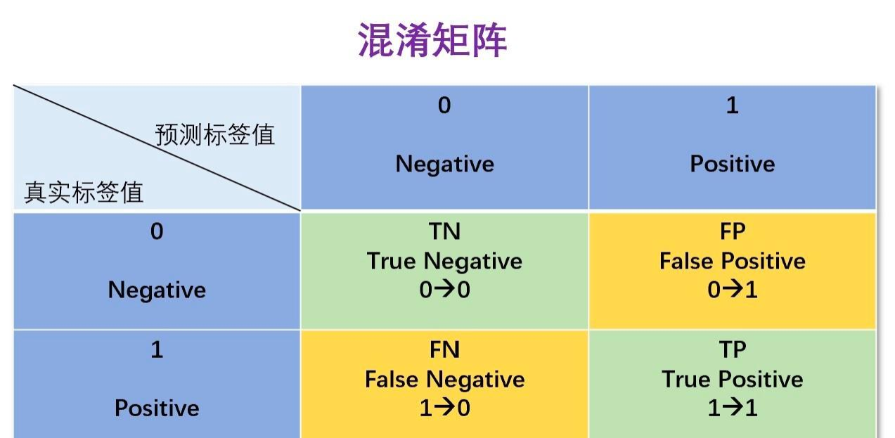
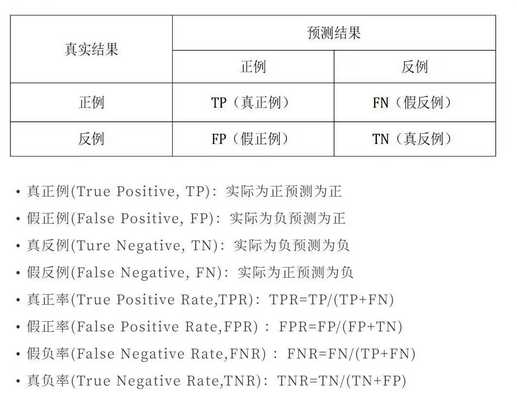
混淆矩阵
在机器学习领域,混淆矩阵(ConfusionMatrix),又称为可能性矩阵或错误矩阵。混淆矩阵的每一列代表了预测类别,每一行代表了数据的真实类别。分类问题的评价指标大多基于混淆矩阵计算得到的。
### 3.confusion_matrix
from sklearn import datasets
from sklearn.svm import LinearSVC
from sklearn.model_selection import cross_validate
from sklearn.metrics import confusion_matrix,ConfusionMatrixDisplay
import matplotlib.pyplot as plt
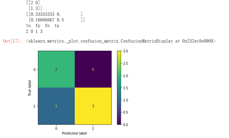
y_true = [1, 0, 1, 1, 0, 1]
y_pred = [0, 0, 1, 1, 0, 1]
cm=confusion_matrix(y_true, y_pred)
print(confusion_matrix(y_true, y_pred))
print(confusion_matrix(y_true, y_pred,normalize='all'))
tn, fp, fn, tp = confusion_matrix(y_true, y_pred).ravel()
print("tn fp fn tp")
print(tn, fp, fn, tp)
disp = ConfusionMatrixDisplay(confusion_matrix=cm)
disp.plot()
# plt.show()输出为:
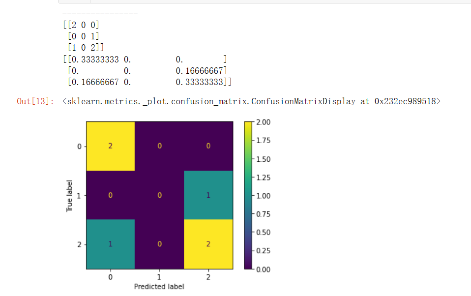
print("----------------")
y_true = [2, 0, 2, 2, 0, 1]
y_pred = [0, 0, 2, 2, 0, 2]

cm=confusion_matrix(y_true, y_pred)
print(confusion_matrix(y_true, y_pred))
print(confusion_matrix(y_true, y_pred,normalize='all'))
disp = ConfusionMatrixDisplay(confusion_matrix=cm)
disp.plot()
# plt.show()
输出为:
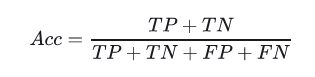
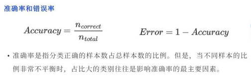
准确率(Accuracy)
识别对了的正例(TP)与负例(TN)占总识别样本的比例。 缺点:类别比例不均衡时影响评价效果。
import numpy as np
from sklearn.metrics import accuracy_score
y_pred = [0, 2, 1, 3]
y_true = [0, 1, 2, 3]
print(accuracy_score(y_true, y_pred)) # 0.5
print(accuracy_score(y_true, y_pred, normalize=False)) # 2
精确率(Precision)
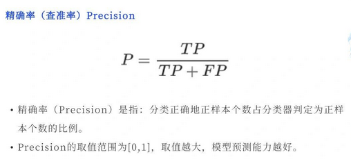
识别正确的正例(TP)占识别结果为正例(TP+FP)的比例。
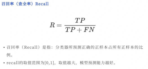
召回率(Recall)
识别正确的正例(TP)占实际为正例(TP+FN)的比例。
通常在排序问题中,采用Top N返回结果的精确率和召回率来衡量排序模型的性能,表示为Precision@N 和Recall@N。 Precision和Recall是一对矛盾又统一的指标,当分类阈值越高时,模型的精确率越高,相反召回率越低。
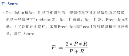
F1值
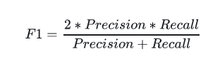
F1是召回率R和精度P的加权调和平均,顾名思义即是为了调和召回率R和精度P之间增减反向的矛盾,对R和P进行加权调和。
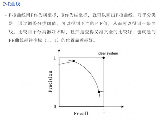
P-R曲线
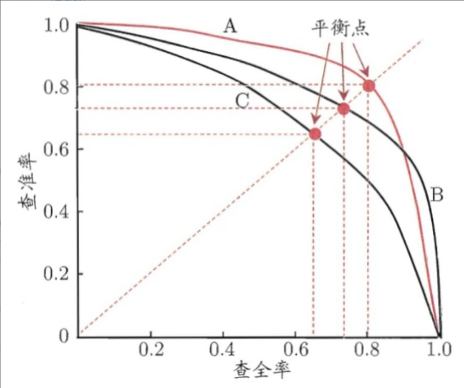
PR曲线通过取不同的分类阈值,分别计算当前阈值下的模型P值和R值,以P值为纵坐标,R值为横坐标,将算得的一组P值和R值画到坐标上,就可以得到P-R曲线。当一个模型的P-R曲线完全包住另一个模型的P-R曲线,则前者的性能优于后者(如A>C,B>C)。
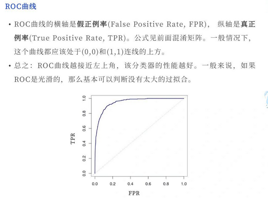
ROC(Receiver Operating Characteristic)
ROC曲线也称受试者工作特征。以FPR(假正例率:假正例占所有负例的比例)为横轴,TPR(召回率)为纵轴,绘制得到的曲线就是ROC曲线。与PR曲线相同,曲线下方面积越大,其模型性能越好。
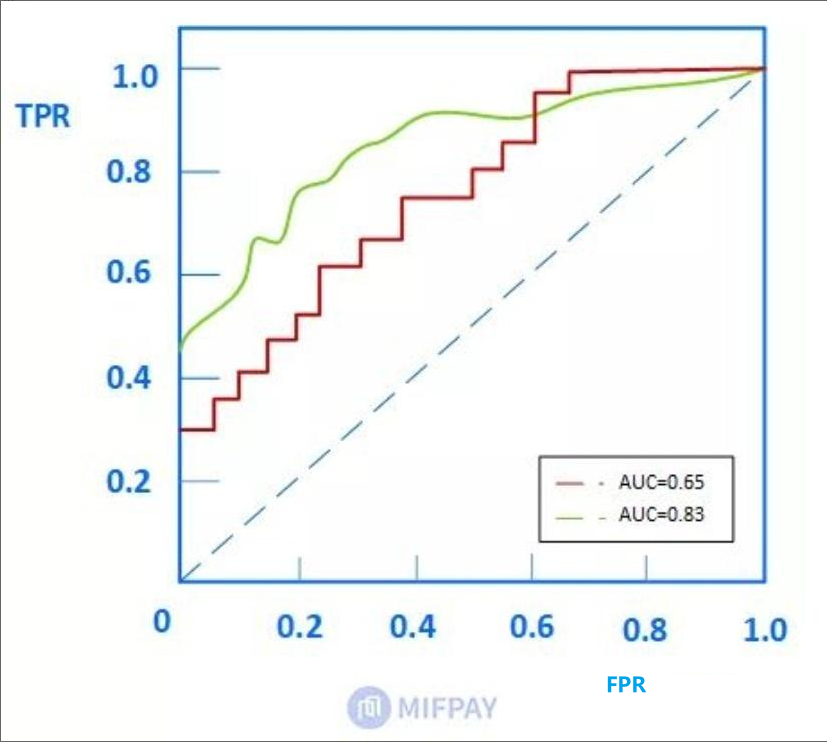
AUC
含义一:ROC曲线下的面积即为AUC。面积越大代表模型的分类性能越好。
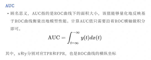
含义二:随机挑选一个正样本以及负样本,算法将正样本排在所有负样本前面的概率就是AUC值。 是排序模型中最为常见的评价指标之一。
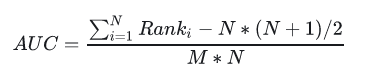
M代表数据集中正样本的数量,N代表负样本数量。AUC的评价效果不受正负样本比例的影响。因为改变正负样本比例,AOC曲线中的横纵坐标大小同时变化,整体面积不变。
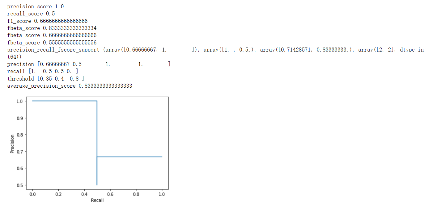
sklearn案例
from sklearn import metrics
y_pred = [0, 1, 0, 0]
y_true = [0, 1, 0, 1]
print("precision_score",metrics.precision_score(y_true, y_pred)) # 1.0
print("recall_score",metrics.recall_score(y_true, y_pred)) #0.5
print("f1_score",metrics.f1_score(y_true, y_pred) )#0.66...
print("fbeta_score",metrics.fbeta_score(y_true, y_pred, beta=0.5)) #0.83...
print("fbeta_score",metrics.fbeta_score(y_true, y_pred, beta=1)) #0.66...
print("fbeta_score",metrics.fbeta_score(y_true, y_pred, beta=2)) #0.55...
print("precision_recall_fscore_support",metrics.precision_recall_fscore_support(y_true, y_pred, beta=0.5) )
#(array([ 0.66..., 1. ]), array([ 1. , 0.5]), array([ 0.71..., 0.83...]), array([2, 2]...))
import numpy as np
from sklearn.metrics import precision_recall_curve
from sklearn.metrics import average_precision_score
y_true = np.array([0, 0, 1, 1])
y_scores = np.array([0.1, 0.4, 0.35, 0.8])
precision, recall, threshold = precision_recall_curve(y_true, y_scores)

# from sklearn.metrics import precision_recall_curve
from sklearn.metrics import PrecisionRecallDisplay

pr_display = PrecisionRecallDisplay(precision=precision, recall=recall).plot()

print("precision",precision) # array([ 0.66..., 0.5 , 1. , 1. ])
print("recall",recall) #array([ 1. , 0.5, 0.5, 0. ])
print("threshold",threshold) #array([ 0.35, 0.4 , 0.8 ])
print("average_precision_score",average_precision_score(y_true, y_scores)) #0.79...
输出为:
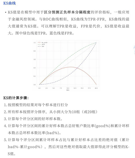
KS曲线
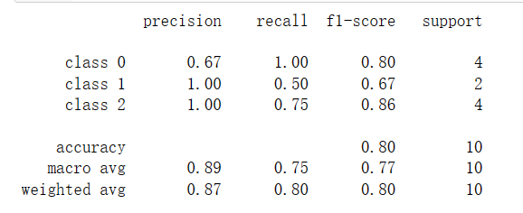
分类报告
from sklearn.metrics import classification_report
y_true = [0, 1, 2, 2, 0,0, 1, 2, 2, 0]
y_pred = [0, 0, 2, 2, 0,0, 1, 2, 0, 0]
target_names = ['class 0', 'class 1', 'class 2']
print(classification_report(y_true, y_pred, target_names=target_names))
输出为:
回归任务
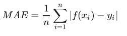
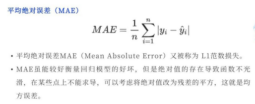
MAE(Mean Absolute Error)
MAE是平均绝对误差,又称L1范数损失。通过计算预测值和真实值之间的距离的绝对值的均值,来衡量预测值与真实值之间的真实距离。
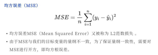
MSE(Mean Square Error)
MSE是真实值与预测值的差值的平方然后求和平均。通过平方的形式便于求导,所以常被用作线性回归的损失函数。
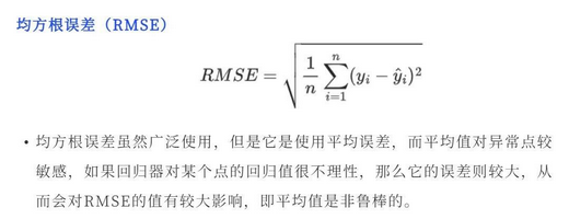
RMSE(Root Mean Square Error)
RMSE衡量观测值与真实值之间的偏差。常用来作为机器学习模型预测结果衡量的标准。 受异常点影响较大,鲁棒性比较差。
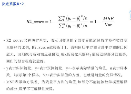
决定系数
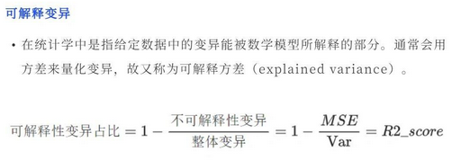
可解释变异
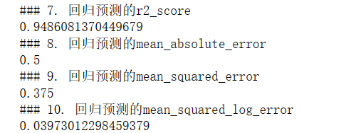
sklearn实现
print("### 7. 回归预测的r2_score ")
# r2_score函数计算决定系数,通常表示为R²。
# 它表示模型中自变量所解释的方差(Y)的比例。它提供了拟合度的指示,
# 因此通过解释方差的比例来衡量未见过的样本可能被模型预测的程度。

from sklearn.metrics import r2_score
y_true = [3, -0.5, 2, 7]
y_pred = [2.5, 0.0, 2, 8]
print(r2_score(y_true, y_pred))

print("### 8. 回归预测的mean_absolute_error")
from sklearn.metrics import mean_absolute_error
y_true = [3, -0.5, 2, 7]
y_pred = [2.5, 0.0, 2, 8]
print(mean_absolute_error(y_true, y_pred))

print("### 9. 回归预测的mean_squared_error ")
from sklearn.metrics import mean_squared_error
y_true = [3, -0.5, 2, 7]
y_pred = [2.5, 0.0, 2, 8]
print(mean_squared_error(y_true, y_pred))

print("### 10. 回归预测的mean_squared_log_error")
from sklearn.metrics import mean_squared_log_error
y_true = [3, 5, 2.5, 7]
y_pred = [2.5, 5, 4, 8]
print(mean_squared_log_error(y_true, y_pred))
输出为:
排序任务
AUC
同上。AUC不受数据的正负样本比例影响,可以准确的衡量模型的排序能力,是推荐算法、分类算法常用的模型评价指标。
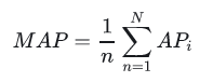
MAP(Mean Average Precision)
全局平均准确率,其中AP表示单用户TopN推荐结果的平均准确率。
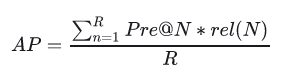
这里R表示推荐的结果序列长度,rel(N)表示第N个推荐结果的相关性分数,这里命中为1,未命中为0。AP衡量的是整个排序的平均质量。对全局所有用户的AP取平均值就是MAP。
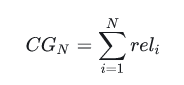
NDCG
首先介绍CG(累计收益),模型会给推荐的每个item打分表示与当前用户的相关性。假设当前推荐item的个数为N个,我们把这N个item的相关分数进行累加,就是当前用户的累积增益:
显然CG不考虑不同位置对排序效果的影响,所以在此基础上引入位置影响因素,即DCG(折损累计增益),位置靠后的结果进行加权处理:
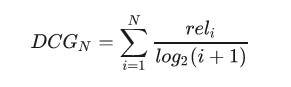
推荐结果的相关性越大,DCG越大,推荐效果越好。
NDCG(归一化折损累计增益),表示推荐系统对所有用户推荐结果DCG的一个平均值,由于每个用户的排序列表不一样,所以先对每个用户的DCG进行归一化,再求平均。其归一化时使用的分母就是IDCG,指推荐系统为某一用户返回的最好推荐结果列表,即假设返回结果按照相关性排序,最相关的结果放在前面,此序列的DCG为IDCG。
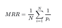
MRR(Mean Reciprocal Rank)
MRR平均倒数排名,是一个国际上通用的对搜索算法进行评价的机制,即第一个结果匹配,分数为1,第二个匹配分数为0.5,第n个匹配分数为1/n,如果没有匹配的句子分数为0。最终的分数为所有得分之和。
聚类任务
聚类任务的评价指标分为内部指标(无监督数据)和外部指标(有监督数据)。
内部指标(无监督数据,利用样本数据与聚类中心之间的距离评价):
紧密度(Compactness)
每个聚类簇中的样本点到聚类中心的平均距离。紧密度越小,表示簇内的样本点越集中,样本点之间聚类越短,也就是说簇内相似度越高。
分割度(Seperation)
每个簇的簇心之间的平均距离。分割度值越大说明簇间间隔越远,分类效果越好,即簇间相似度越低。
轮廓系数 (Silhouette Coefficient)
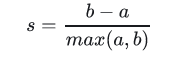
对于一个样本集合,它的轮廓系数是所有样本轮廓系数的平均值。轮廓系数的取值范围是[-1,1],同类别样本距离越相近,不同类别样本距离越远分数越高。假设:
a:某个样本与其所在簇内其他样本的平均距离
b:某个样本与其他簇样本的平均距离
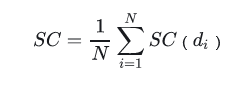
单个样本的轮廓系数s为:
聚类的总体轮廓系数为:
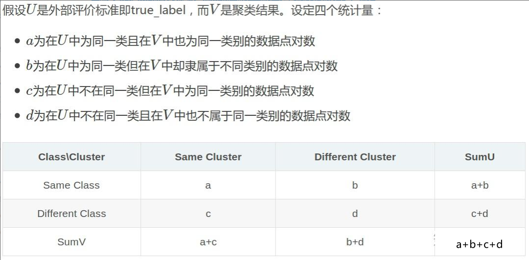
外部指标(有监督数据,利用样本数据与真实label进行比较评价):
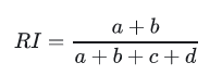
兰德系数(Rand index)
兰德系数是使用真实label对聚类效果进行评估,评估过程和混淆矩阵的计算类似:
互信息(Mutual Information)
sklearn实现聚类
print("### 11.无监督聚类的Silhouette Coefficient")
from sklearn import metrics
from sklearn import datasets
import numpy as np
X, y = datasets.load_iris(return_X_y=True)

from sklearn.cluster import KMeans
kmeans_model = KMeans(n_clusters=3, random_state=1).fit(X)
labels = kmeans_model.labels_
print(metrics.silhouette_score(X, labels, metric='euclidean'))
输出为:
11.无监督聚类的Silhouette Coefficient 0.5528190123564091
完整代码
from sklearn import metrics
# 查看模块的函数
dir(metrics)
print("### 1.Accuracy score")
import numpy as np
from sklearn.metrics import accuracy_score
y_pred = [0, 2, 1, 3]
y_true = [0, 1, 2, 3]
print(accuracy_score(y_true, y_pred))
print(accuracy_score(y_true, y_pred, normalize=False)) # 正确的预测个数
print("### 2.Top-k accuracy score")
# top_k_accuracy_score函数是accuracy_score的泛化。
# 区别在于,只要真实标签与k个最高预测分数之一相关联,预测就被认为是正确的。
# 准确度_分数是k=1的特殊情况。
import numpy as np
from sklearn.metrics import top_k_accuracy_score
y_true = np.array([0, 1, 2, 2])
y_score = np.array([[0.5, 0.2, 0.2],
[0.3, 0.4, 0.2],
[0.2, 0.4, 0.3],
[0.7, 0.2, 0.1]])
print(top_k_accuracy_score(y_true, y_score, k=2))
# Not normalizing gives the number of "correctly" classified samples
print(top_k_accuracy_score(y_true, y_score, k=2, normalize=False))
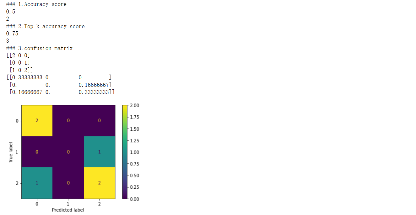
print("### 3.confusion_matrix")
from sklearn import datasets
from sklearn.svm import LinearSVC
from sklearn.model_selection import cross_validate
from sklearn.metrics import confusion_matrix,ConfusionMatrixDisplay
import matplotlib.pyplot as plt
y_true = [2, 0, 2, 2, 0, 1]
y_pred = [0, 0, 2, 2, 0, 2]
cm=confusion_matrix(y_true, y_pred)
print(confusion_matrix(y_true, y_pred))
print(confusion_matrix(y_true, y_pred,normalize='all'))
disp = ConfusionMatrixDisplay(confusion_matrix=cm)
disp.plot()
plt.show()
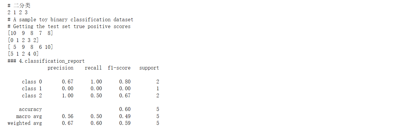
print("# 二分类")
y_true = [0, 0, 0, 1, 1, 1, 1, 1]
y_pred = [0, 1, 0, 1, 0, 1, 0, 1]
tn, fp, fn, tp = confusion_matrix(y_true, y_pred).ravel()
print(tn, fp, fn, tp)
print("# A sample toy binary classification dataset")
X, y = datasets.make_classification(n_classes=2, random_state=0)
svm = LinearSVC(random_state=0)
def confusion_matrix_scorer(clf, X, y):
y_pred = clf.predict(X)
cm = confusion_matrix(y, y_pred)
return {'tn': cm[0, 0], 'fp': cm[0, 1],
'fn': cm[1, 0], 'tp': cm[1, 1]}
cv_results = cross_validate(svm, X, y, cv=5,
scoring=confusion_matrix_scorer)
print("# Getting the test set true positive scores")
print(cv_results['test_tp'])
# Getting the test set false negative scores
print(cv_results['test_fn'])
print(cv_results['test_tn'])
print(cv_results['test_fp'])
print("### 4.classification_report")
from sklearn.metrics import classification_report
y_true = [0, 1, 2, 2, 0]
y_pred = [0, 0, 2, 1, 0]
target_names = ['class 0', 'class 1', 'class 2']
print(classification_report(y_true, y_pred, target_names=target_names))
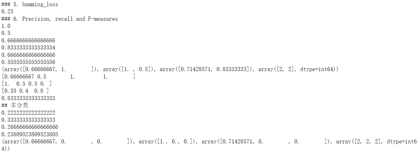
print("### 5. hamming_loss")
from sklearn.metrics import hamming_loss
y_pred = [1, 2, 3, 4]
y_true = [2, 2, 3, 4]
print(hamming_loss(y_true, y_pred))
print("### 6. Precision, recall and F-measures")
from sklearn import metrics
y_pred = [0, 1, 0, 0]
y_true = [0, 1, 0, 1]
print(metrics.precision_score(y_true, y_pred))
print(metrics.recall_score(y_true, y_pred))
print(metrics.f1_score(y_true, y_pred))
print(metrics.fbeta_score(y_true, y_pred, beta=0.5))
print(metrics.fbeta_score(y_true, y_pred, beta=1))
print(metrics.fbeta_score(y_true, y_pred, beta=2))
print(metrics.precision_recall_fscore_support(y_true, y_pred, beta=0.5))
import numpy as np
from sklearn.metrics import precision_recall_curve
from sklearn.metrics import average_precision_score
y_true = np.array([0, 0, 1, 1])
y_scores = np.array([0.1, 0.4, 0.35, 0.8])
precision, recall, threshold = precision_recall_curve(y_true, y_scores)
print(precision)
print(recall)
print(threshold)
print( average_precision_score(y_true, y_scores))
print("## 多分类")
from sklearn import metrics
y_true = [0, 1, 2, 0, 1, 2]
y_pred = [0, 2, 1, 0, 0, 1]
print(metrics.precision_score(y_true, y_pred, average='macro'))
print(metrics.recall_score(y_true, y_pred, average='micro'))
print(metrics.f1_score(y_true, y_pred, average='weighted'))
print(metrics.fbeta_score(y_true, y_pred, average='macro', beta=0.5))
print(metrics.precision_recall_fscore_support(y_true, y_pred, beta=0.5, average=None))
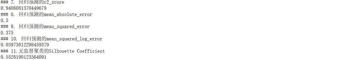
print("### 7. 回归预测的r2_score ")
# r2_score函数计算决定系数,通常表示为R²。
# 它表示模型中自变量所解释的方差(Y)的比例。它提供了拟合度的指示,
# 因此通过解释方差的比例来衡量未见过的样本可能被模型预测的程度。
from sklearn.metrics import r2_score
y_true = [3, -0.5, 2, 7]
y_pred = [2.5, 0.0, 2, 8]
print(r2_score(y_true, y_pred))
print("### 8. 回归预测的mean_absolute_error")
from sklearn.metrics import mean_absolute_error
y_true = [3, -0.5, 2, 7]
y_pred = [2.5, 0.0, 2, 8]
print(mean_absolute_error(y_true, y_pred))
print("### 9. 回归预测的mean_squared_error ")
from sklearn.metrics import mean_squared_error
y_true = [3, -0.5, 2, 7]
y_pred = [2.5, 0.0, 2, 8]
print(mean_squared_error(y_true, y_pred))
print("### 10. 回归预测的mean_squared_log_error")
from sklearn.metrics import mean_squared_log_error
y_true = [3, 5, 2.5, 7]
y_pred = [2.5, 5, 4, 8]
print(mean_squared_log_error(y_true, y_pred))
print("### 11.无监督聚类的Silhouette Coefficient")
from sklearn import metrics
from sklearn import datasets
import numpy as np
X, y = datasets.load_iris(return_X_y=True)
from sklearn.cluster import KMeans
kmeans_model = KMeans(n_clusters=3, random_state=1).fit(X)
labels = kmeans_model.labels_
print(metrics.silhouette_score(X, labels, metric='euclidean'))输出为:
目标函数、损失函数、代价函数、评价函数区别
在机器学习和优化问题中,目标函数、损失函数、代价函数都是评估和优化模型的关键概念,它们之间既有联系又有区别:
- 损失函数(Loss Function):
- 描述了一个模型对于单个样本预测输出与真实值之间的差异。损失函数通常是非负的,并且理想情况下,在预测完全准确时其值为零。
- 举例:在二元分类问题中,常用的损失函数包括逻辑回归的对数损失(Log Loss, Binary Cross-Entropy Loss),它量化了模型预测的概率分布与实际标签之间的距离。
- 代价函数(Cost Function):
- 在机器学习中,特别是在监督学习场景下,代价函数指的是在整个训练集上的损失函数的平均值,即所有样本损失之和的平均,用来衡量模型在所有训练数据上的整体表现。
- 举例:假设我们在做线性回归,使用的损失函数可能是每个样本的平方误差,代价函数则是所有样本平方误差之和除以样本数量,即均方误差(Mean Squared Error, MSE)。
- 目标函数(Objective Function):
- 目标函数是模型优化过程中试图最小化的函数,它不仅包含训练误差的部分(如代价函数),还可能包含正则化项(Regularization Term),旨在控制模型复杂度,防止过拟合。
- 举例:在线性回归中,目标函数可能是代价函数加上L1或L2正则化项,如岭回归(Ridge Regression)的目标函数是在MSE的基础上添加了权重向量的L2范数惩罚项。
总结一下:
- 损失函数关注单个数据点的预测误差;
- 代价函数是损失函数在训练集上的平均,反映了模型在所有训练数据上的总体性能;
- 目标函数进一步扩展了代价函数的概念,包含了对模型复杂性的惩罚项,体现了模型泛化能力的考量。
在不同的文献和上下文中,有时人们会互换使用“代价函数”和“损失函数”的说法,尤其是在只考虑训练误差而不涉及正则化时。而在正则化存在的情况下,目标函数则明确包含了正则化项,是优化过程中真正要最小化的目标。
- 评价函数: 损失函数是用来衡量预测值和真实值差距的函数,是模型优化的目标,所以也称之目标函数、优化评分函数。这是机器学习中很重要的性能衡量指标。 评价函数和损失函数相似,只是关注点不同: 损失函数用于训练过程, 而评价函数用于模型训练完成后(或每一批次训练完成后)的度量,
确定方向过程
针对完全没有基础的同学们 1.确定机器学习的应用领域有哪些 2.查找机器学习的算法应用有哪些 3.确定想要研究的领域极其对应的算法 4.通过招聘网站和论文等确定具体的技术 5.了解业务流程,查找数据 6.复现经典算法 7.持续优化,并尝试与对应企业人员沟通心得 8.企业给出反馈