[ncb图表复现] ggplot2绘制多层分组热图
[ncb图表复现] ggplot2绘制多层分组热图

R语言数据分析指南
发布于 2023-12-26 18:51:27
发布于 2023-12-26 18:51:27
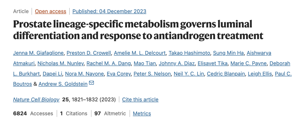
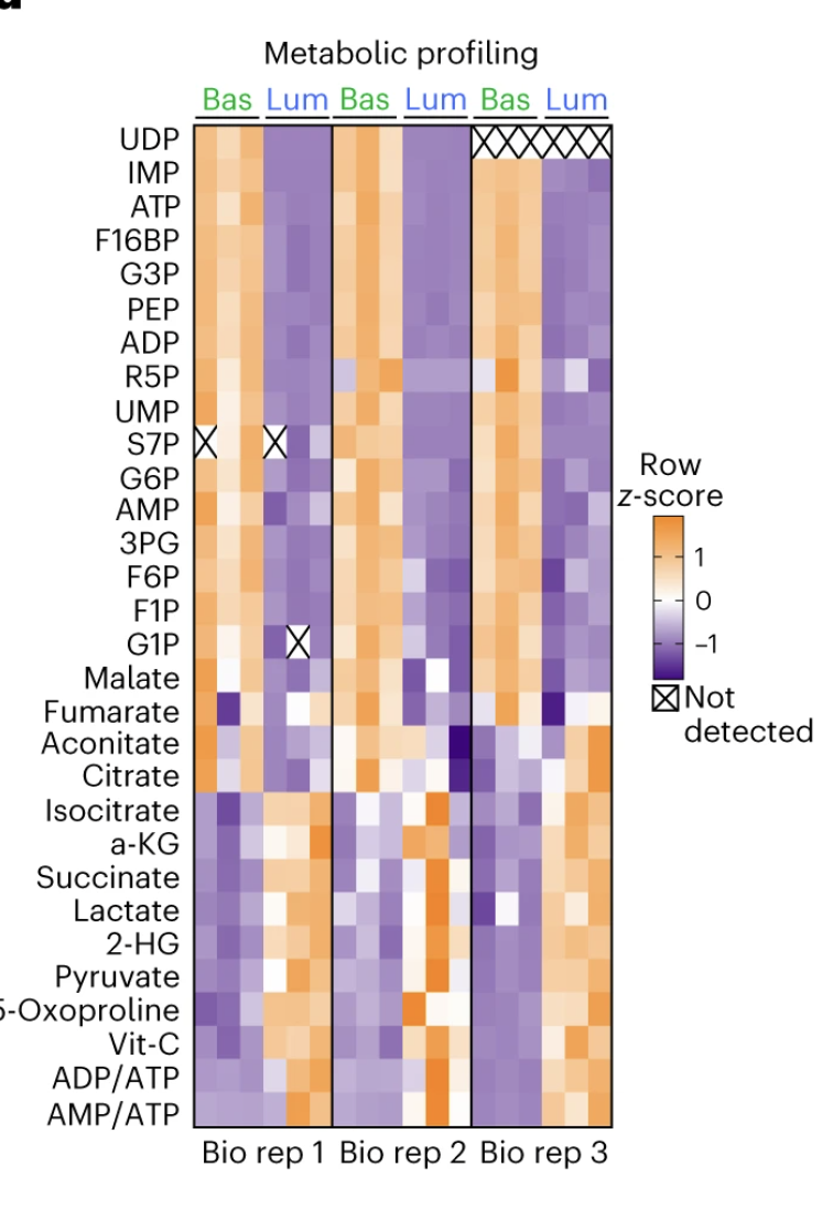
❝本节来复现nature cell biology上的一张热图,通过一系列数据清洗来介绍图形细节的调整,整个过程仅参考。希望对各位观众老爷能有所帮助。「数据代码已经整合上传到2023VIP交流群」,加群的观众老爷可自行下载,有需要的朋友可关注文末介绍加入VIP交流群。 ❞
论文
加载R包
library(tidyverse)
library(ggh4x)
library(MetBrewer)
数据清洗
df <- read_tsv("data.tsv") %>% pivot_longer(-gene) %>%
  extract(col = name, into ="group1",regex = "([^\\s]+).*",remove = FALSE) %>%
  mutate(group1=case_when(group1=="Basal" ~ "Bas",
                         group1=="Luminal" ~ "Lum")) %>%
  mutate(group2 = case_when(
    grepl("1-.", name) ~ "Bio rep 1",
    grepl("2-.", name) ~ "Bio rep 2",
    grepl("3-.", name) ~ "Bio rep 3",
    TRUE ~ "Other"
  ))
数据可视化
df %>%
  ggplot(.,aes(interaction(name,group1),gene,color=value,fill=value))+
  geom_tile()+
  facet_grid(.~group2,scales = "free_x",switch = "x")+
  guides(x="axis_nested")+
  scale_x_discrete(expand=c(0,0),position = 'top')+
  scale_y_discrete(expand=c(0,0))+
  scale_fill_gradientn(colors=met.brewer("Cassatt1"),na.value = NA)+
  scale_color_gradientn(colors=met.brewer("Cassatt1"),na.value = NA)+
  labs(x=NULL,y=NULL,fill="Row \n z-score",color="Row \n z-score") +
  theme(axis.text.x=element_blank(),
        axis.text.y=element_text(color="black",size=8,face="italic"),
        axis.ticks.x=element_blank(),
        axis.ticks.y=element_blank(),
        strip.background = element_blank(),
        strip.text = element_text(color="black",size=9,face="bold"),
        panel.background = element_blank(),
        plot.background = element_blank(),
        legend.spacing.x = unit(0.1,"cm"),
        panel.spacing.x =unit(0.01,"cm"),
        panel.border=element_rect(fill=NA,color="black",size=0.5,linetype="solid"),
        ggh4x.axis.nestline.x = element_line(size=0.5,color="black"),
        ggh4x.axis.nesttext.x = element_text(colour ="black",angle=0,size=10,vjust=0,hjust=0.5,face="bold",
                                             margin = margin(b=3)),
        plot.margin=unit(c(0.2,0.2,0.2,0.2),units=,"cm"))
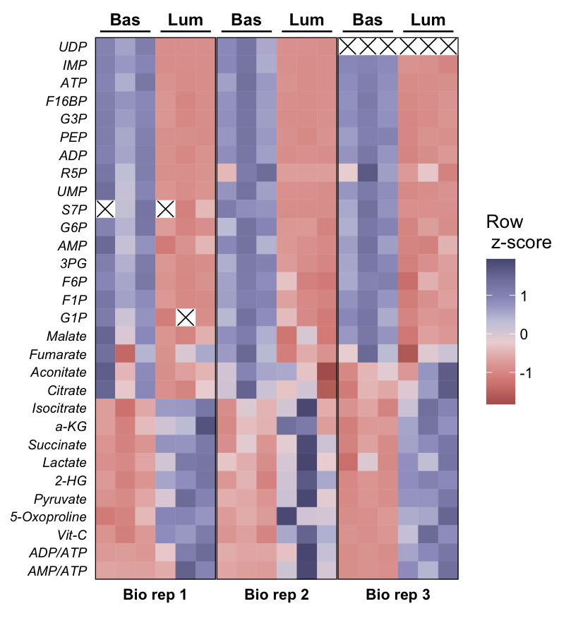
复现图
本文参与 腾讯云自媒体分享计划,分享自微信公众号。
原始发表:2023-12-23,如有侵权请联系 cloudcommunity@tencent.com 删除
评论
登录后参与评论
推荐阅读
目录