细胞通讯分析之CellphoneDB（二）可视化篇

生信菜鸟团

发布于 2023-01-05 21:13:17

5.1K0

发布于 2023-01-05 21:13:17

时间过得好快，又一个月过去了！前几期我分享了CellChat的学习笔记，包括：

在此基础上，我还写了CellphoneDB的笔记：细胞通讯分析之CellphoneDB初探（一），在这个帖子里简单介绍了CellphoneDB，以及CellphoneDB的环境配制、单样本实战，最后提供了一个可视化的函数cellphoneDB_Dotplot。另外，cellphoneDB似乎是不支持小鼠等其他物种的数据，因此我写了 一行代码完成单细胞数据人鼠基因同源转换，提供了一个函数，一行代码完成人鼠的基因同源转换，然后用转换后的数据走cellphoneDB流程即可。

本期的帖子接上文，主要解决CellphoneDB的2个问题：

由于目前一个单细胞项目基本包含数个/数十个样本，如何实现CellphoneDB的批量处理；
实现更多更丰富的可视化。

一. CellphoneDB的批量处理

1.1 首先在R语言环境下输出表达数据及表型数据：

library(Seurat)
library(tidyverse)
library(data.table)
library(dplyr)
library(readr)

#### 1.load data
scRNA = read_rds("./Step4.m.seurat.rds")

#### 2.批量输出Output
out.dir = "Step8.CellphoneDB/"
for(sample in unique(scRNA$sampleID)){
  sp1 <- subset(scRNA,sampleID == sample)
  sp1_counts <- as.data.frame(sp1@assays$RNA@data) %>% 
    rownames_to_column(var = "Gene")
  
  sp1_meta <- data.frame(Cell=rownames(sp1@meta.data), 
                         cell_type=sp1@meta.data$celltype)
  
  fwrite(sp1_counts,file = paste0(out.dir,sample,"_counts.txt"), row.names=F, sep='\t')
  fwrite(sp1_meta, file = paste0(out.dir,sample,"_meta.txt"), row.names=F, sep='\t')
}

运行之后out.dir目录下就会生成每个样本的表达数据和meta表型数据的txt文件。

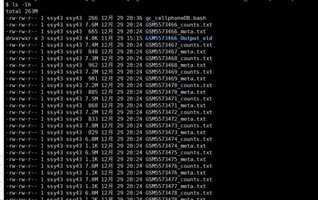
然后在Linux环境下批量运行CellphoneDB：

1.2 首先写一个通用型的shell脚本

##进入目的文件夹
cd Step8.CellphoneDB/

##先写个脚本
cat >gc_cellphoneDB.bash
file_count=./$1_counts.txt
file_anno=./$1_meta.txt
outdir=./$1_Output

if [ ! -d ${outdir} ]; then
mkdir ${outdir}
fi
cellphonedb method statistical_analysis ${file_anno} ${file_count} --counts-data hgnc_symbol --output-path ${outdir} --threshold 0.01 --threads 10 
##如果细胞数太多，可以添加下采样参数，默认只分析1/3的细胞
#--subsampling
#--subsampling-log true #对于没有log转化的数据，还要加这个参数

1.3 然后批量运行

##激活环境
conda activate cpdb 

##批量运行此脚本
ls *counts.txt | while read id;
do 
id=${id%%_counts.txt}
echo $id
bash gc_cellphoneDB.bash $id 1>${id}.log 2>&1 
done

每个样本的结果在当前目录下。

二. CellphoneDB的多种可视化方案

除了我上期用健明老师的代码改编的函数cellphoneDB_Dotplot绘制气泡图（详见细胞通讯分析之CellphoneDB初探（一）），我们还可以使用如下方案进行可视化。

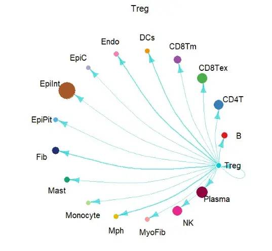
2.1 衔接Cellchat的函数

其实只要深刻理解Cellchat这个包的函数逻辑，我们即可用cellphoneDB的结果作为input数据，进行可视化。

这里需要的文件是count_network.txt作为input数据。

library(CellChat)
library(tidyr)
df.net <- read.table("./Step8.CellphoneDB/GSM5573466_Output/Outplot/count_network.txt",
                     header = T,sep = "\t",stringsAsFactors = F)
meta.data <- read.table("./Step8.CellphoneDB/GSM5573466_meta.txt",
                        header = T,sep = "\t",stringsAsFactors = F)

groupSize <- as.numeric(table(meta.data$cell_type))

df.net <- spread(df.net, TARGET, count)
rownames(df.net) <- df.net$SOURCE
df.net <- df.net[, -1]
df.net <- as.matrix(df.net)

netVisual_circle(df.net, vertex.weight = groupSize,
                 weight.scale = T, label.edge= F,
                 title.name = "Number of interactions")

image-20221229204130690

# par(mfrow = c(3,3), xpd=TRUE)
for (i in 1:nrow(df.net)) {
  mat2 <- matrix(0, nrow = nrow(df.net), ncol = ncol(df.net), dimnames = dimnames(df.net))
  mat2[i, ] <- df.net[i, ]
  
  netVisual_circle(mat2, 
                   vertex.weight = groupSize,
                   weight.scale = T, 
                   edge.weight.max = max(df.net),
                   title.name = rownames(df.net)[i],
                   arrow.size=0.5)
  
}

批量输出互作结果，这里只显示其中1个：

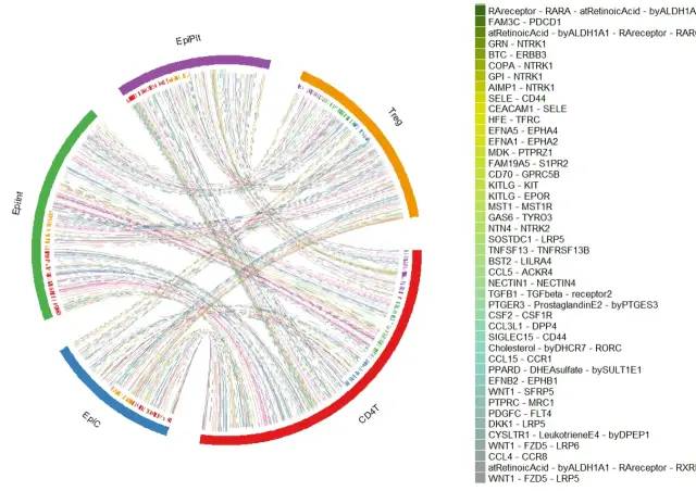
2.2 R包ktplots

参考追风哥在简书上写的笔记：10X单细胞 && 10X空间转录组分析之cellphoneDB可视化进阶，github: https://github.com/zktuong/ktplots。这个包自带了非常多的可视化方案，这里列举其中一两种：

#devtools::install_github('zktuong/ktplots', dependencies = TRUE)
library(ktplots)
library(Seurat)
library(SingleCellExperiment)
library(tidyverse)
library(data.table)
library(dplyr)
library(readr)

#### 1 加载数据
mypvals <- read.table("./Step8.CellphoneDB/GSM5573466_Output/pvalues.txt",header = T,sep = "\t",stringsAsFactors = F,check.names = F)
mymeans <- read.table("./Step8.CellphoneDB/GSM5573466_Output/means.txt",header = T,sep = "\t",stringsAsFactors = F,check.names = F) 
mydecon <- read.table("./Step8.CellphoneDB/GSM5573466_Output/deconvoluted.txt",header = T,sep = "\t",stringsAsFactors = F,check.names = F)

#单细胞数据
seurat.data = read_rds("./Step4.m.seurat.rds")
scRNA =  subset(seurat.data,sampleID == "GSM5573466")
table(scRNA$celltype)
#Seurat转SCE
sce <- Seurat::as.SingleCellExperiment(scRNA)

## Vis 1
p1 <- plot_cpdb3(cell_type1 = 'CD4T|Treg', 
                 cell_type2 = 'EpiC|EpiInt|EpiPit',
                 scdata = sce,
                 idents = 'celltype', # column name where the cell ids are located in the metadata
                 means = mymeans,
                 pvals = mypvals,
                 deconvoluted = mydecon, # new options from here on specific to plot_cpdb3
                 keep_significant_only = TRUE,
                 standard_scale = TRUE,
                 remove_self = TRUE,
                 legend.pos.x = -5,legend.pos.y = 5
)
p1

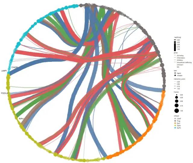
再复杂一点的：

p2 <- plot_cpdb2(cell_type1 = "CD4T|Treg", # same usage style as plot_cpdb
 cell_type2 = 'EpiC|EpiInt|EpiPit',
 idents = 'celltype',
 scdata = sce,
 means = mymeans,
 pvals = mypvals,
 deconvoluted = mydecon, # new options from here on specific to plot_cpdb2
 desiredInteractions = list(c('CD4T', 'Treg'), c('Treg', 'EpiC'), c('Treg', 'EpiInt'), c('Treg', 'EpiPit')),
 interaction_grouping = interaction_annotation,
    edge_group_colors = c("Activating" = "#e15759", "Chemotaxis" = "#59a14f", "Inhibitory" = "#4e79a7", "Intracellular trafficking" = "#9c755f", "DC_development" = "#B07aa1"),
    node_group_colors = c("CD4T" = "#86bc86", "Treg" = "#79706e", "EpiC" = "#ff7f0e", "EpiInt" = "#bcbd22"  ,"EpiPit" = "#17becf"),
    keep_significant_only = TRUE,
    standard_scale = TRUE,
    remove_self = TRUE)
p2